Euro-SiBRAM’2002 Prague, June 24 to 26, 2002, Czech Republic

Session 3

Database-Assisted Design for Wind Loading

Emil Simiu¹, Fahim Sadek¹, Timothy M. Whalen², Seokkwon Jang³, Le-Wu Lu³, Sofia M.C. Diniz⁴, Andrea Grazini⁵, and Michael A. Riley¹

¹Building and Fire Research Laboratory, National Institute of Standards and Technology,

Gaithersburg, MD 20899-8611, USA, ph. 301 975-6076, fax 301 869-6275, emil.simiu@nist.gov

²School of Civil Engineering, Purdue University, West Lafayette, IN 47907-1284, USA

³Department of Civil Engineering, Lehigh University, Bethlehem, PA 18015, USA

⁴Federal University of Minas Gerais, Belo Horizonte, MG 30110-060, Brazil

⁵Department of Civil Engineering, University of Perugia, 61025 Perugia, Italy

Abstract

Current ASCE Standard provisions on wind loads for low-rise building design are based on wind tunnel tests conducted at the University of Western Ontario in the 1970’s. In spite of the advances they entailed at the time, those provisions are inadequate. UWO tests were conducted at low angular and spatial resolutions. Their results were then used to create drastically simplifying standard aerodynamic tables and plots designed for slide-rule era calculations and entailing errors that can be substantial. These errors can exceed 60 %.

Significant improvements in main wind-load resisting system and component design can be achieved by using database-assisted design (DAD) and associated structural reliability tools, thus accounting realistically for the complexity of the wind loading as well as for the stochasticity and knowledge uncertainties affecting wind effects calculations. We illustrate DAD’s capability to obtain, for the first time in a wind engineering context, realistic estimates of ultimate limit states due to local or global buckling failure. In the future other types of nonlinear behavior associated with ultimate limit states can be similarly dealt with. We note that DAD is ideally suited for use with data likely to be obtained in the future by Computational Fluid Dynamics methods.

Key Words: Building technology, database-assisted design, dynamic response, low-rise buildings, nonlinear behavior, purlins, structural reliability, ultimate limit states, wind loads.

1.         Introduction

1.1              Inadequacy of Current Aerodynamic Standard Provisions

Following Irminger’s 1894 aerodynamic tests it was stated: “It will be due to him that we surely in the future shall save tons of material in our roofs” [1]. Flachsbart’s 1932 boundary layer wind tunnel experiments [2], and University of Western Ontario (UWO) tests sponsored by the Metal Buildings Manufacturers Association (MBMA) in the 1970’s further advanced the state of the art [3].

The technological gap is far wider in wind engineering between 2002 and the 1970’s than between the 1970’s and 1894. In the 1970’s wind pressure measurement, data storage, and data processing capabilities were still relatively primitive. For example, 1970’s UWO tests were conducted predominantly for wind directions in increments of 45°[3]. In contrast, UWO conducted in 1997 [4] and 2001 [5] similar tests in increments of 5°, an order of magnitude improvement. Similar improvements were achieved with respect to numbers of pressure taps per unit area. The low resolution in the tests of [3] is just one reason why the ASCE Standard contains inadequate aerodynamic information. More importantly, it is shown in this paper that the use of the results of [3] to develop, “by eyeball,” drastically simplified aerodynamic tables and plots designed for slide-rule era calculations can lead to errors in the estimation of wind effects in excess of 60 %.

1.2              The Computer Revolution Enables a More Realistic Approach to Wind Load Specification: Database-Assisted, Reliability-Based Design

More than one century after Irminger’s experiments and a quarter of a century after the UWO/MBMA tests, major advances in measurement, data storage, and computational capabilities warrant revision of the methods by which buildings are commonly designed for wind. Improved methods that make use of those capabilities can save large amounts of material, meaning that construction costs and the energy embodied in new construction can be reduced. These methods can also achieve designs resulting in significantly reduced losses from extreme winds, and help to identify weaknesses of existing construction in need of retrofitting.

A modernization of the methods for estimating wind effects is in progress. This will bring computations of wind effects in line with the now routine computer-intensive calculations of internal forces induced by specified loads. Thanks to cooperative efforts by the National Institute of Standards and Technology (NIST), UWO, Purdue University, Texas Tech University (TTU), CECO Building Systems, and MBMA, a pilot project initiated by NIST to develop a computer-intensive, user-friendly design procedure for the calculation of wind effects is now close to completion. The procedure, referred to as database-assisted design (DAD), is complemented by reliability-based modules, and uses the following input:

·      Aerodynamic information. This is supplied by an aerodynamic database containing simultaneous records of time histories of pressure coefficients for as many as 37 wind directions at 500 to 1,000 ports on the exterior and in some cases interior surfaces of the building, for a sufficiently large number of building types and geometries. In this context “sufficient” means larger than the number of building types and geometries used to develop current ASCE 7 Standard provisions. For low-rise industrial buildings with gable roofs, constant eave height, and a rectangular shape in plan, about 15 distinct geometries were tested at UWO in both open and built-up terrain conditions [3]. In view of the improved resolution of the measurements and the absence of “eyeball” summarizing of test results, a new aerodynamic database that would cover the same number of distinct geometries would still lead to improved wind effects calculations. However, this number can easily be exceeded in a future aerodynamic database. For the time being the database – which is being augmented -- covers about 25 geometries, a number sufficient for developmental purposes.

·      Climatological information. To estimate wind effects the procedure can use databases consisting of the extreme wind rosettes (i.e., plots of maximum directional wind speeds) for each of a sufficient number of storms. Currently the climatological database includes rosettes for 999 hurricanes at about 50 equidistant mileposts on the Gulf and Atlantic coastlines [6]; see [7] for accessing information. To our knowledge this is the only open, publicly available hurricane wind speed database. Databases could be developed and/or made available to the public that would cover the entire area of the United States affected by hurricane winds, rather than just the coastline, and would include rosettes associated with more than 999 simulated hurricanes. Where directional wind speed data, simulated or recorded, are not available, the procedure uses wind speeds with specified mean recurrence intervals estimated without regard for wind directionality.

·      Estimates of knowledge uncertainties. This includes estimates based on sample sizes of extreme climatological data, the length and resolution of wind tunnel records, and other information pertaining to the definition of the wind environment.

·      Structural information. For an industrial metal building with portal frames this consists of the distance between frames, the locations, types of support, sizes of purlins and girts, and the cross sections of the frames or the influence lines for the frames’ bending moments, shear forces, and axial forces.

     Software for using the aerodynamic, climatological, and structural information to obtain internal forces is described in [8]. At this time the software covers low-rise buildings that do not exhibit dynamic amplification effects. An extension to flexible buildings is in progress. Added to the software will be an automated procedure, based on results of [9], for interpolation of pressure time histories for buildings with dimensions different from those covered in the database. The software described in [8] has been expanded to include probabilistic modules that provide information on the estimated probability distribution of the peak internal forces for a specified wind speed [10]. A further expansion is in progress, aimed at using this information, as well as statistics of extreme wind speeds and estimates of knowledge uncertainties, to estimate the probability distribution of the wind effects being sought. The knowledge uncertainties pertain to the wind speed or other observations on the basis of which wind speeds may be inferred, terrain roughness, ratios between wind speeds in different roughness regimes, extreme wind speed distribution parameters, ratios between 3-s gusts and the corresponding hourly mean speeds, length of wind tunnel records, wind tunnel performance characteristics, extent to which the wind tunnel reproduces correctly the full-scale aerodynamics, and so forth. The requisite estimates are obtained principally by Monte Carlo simulations, as described in [11, 12]. The software has also been expanded to account for the effects of aerodynamic and climatological wind directionality. The inclusion of comprehensive aerodynamic, climatological, structural, and reliability information and models makes it possible to account in a faithful manner for the complexity of the wind loading, and the stochasticity and knowledge uncertainties inherent in the estimation of wind effects. As the state of the art evolves, model improvements achieved through research can easily be incorporated in DAD for codification, design, retrofitting, and loss estimation purposes.

1.3              Organization of Paper

In Section 2 we show that DAD analyses reveal serious shortcomings of the ASCE 7 Standard, and can achieve significant improvements in the design of main wind-load resisting systems and components (e.g., purlins). In Section 3 we present estimates of nominal wind load factors corresponding to ultimate limit states associated with local and global buckling in portal frames. We show that the factors differ significantly depending upon whether they are based on realistic wind loads estimated by DAD or on the cruder ASCE Standard wind loads. In Section 4 we discuss outstanding codification issues, and ways in which recently developed reliability-based procedures that may be used in conjunction with DAD have contributed and may be expected to contribute to their solution. In Section 5 we mention the possibility of introducing in wind tunnel or Computational Fluid Dynamics aerodynamic databases systematic corrections based on full-scale test results. Section 6 presents our conclusions.

2.         Improved Design of Frames and Components for Wind Loading

2.1       Introduction

In this section we briefly describe the buildings for which aerodynamic data were obtained at the University of Western Ontario and that we use as case studies for the assessment of ASCE 7 Standard provisions (Section 2.2). We show that the assumption in the ASCE 7-98 Standard that aerodynamic coefficients are independent of terrain roughness is significantly in error (Section 2.3). In Section 2.4 we show examples of discrepancies between bending moments in frames calculated by the ASCE 7-98 Standard and on the basis of the UWO data [4].

2.2       Building Descriptions

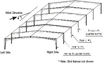
On commission from NIST and NIST/TTU, UWO has conducted comprehensive tests of buildings with gable roofs with 1/24 slopes, plan dimensions 61 m x 30.5 m, and eave heights 6.1 m and 9.75 m in open and suburban terrain [4], and with gable roofs with slopes 1/12, plan dimensions 38.1 m x 24.4 m, and eave height 9.75 m in open terrain [5]. For the set of tests of [4] the total number of pressure taps per building was about 500, and no internal pressures were measured. For the set of [5] the total number of taps per building was 665, with a roof zone of 12 m x 12.2 m for which the number of taps was 135 (i.e., a density of 0.92 taps per square meter). Internal pressures were measured for models with distributed openings causing uniform leakage. The buildings tested in [4] were used as case studies for calculations of internal forces in tapered portal steel frames at 7.62 m o/c (Fig. 1). Like all buildings designed under the aegis of MBMA, the buildings were designed in accordance with the ASCE 7-93 Standard [13] and the AISC 1989 design manual (allowable stress design).

Figure 1.  Isometric view of interior frames

2.3       Dependence of Aerodynamic Coefficients on Terrain Roughness

The ASCE 7-98 Standard [14, p. 42] specifies aerodynamic pressures based on the use of its Fig. 6-4, which is based on the assumption that the aerodynamic coefficients are independent of terrain roughness. Using DAD calculations based on the databases provided by UWO [4] we show that this assumption is incorrect.

     Consider for a given building the ratio

     R_ab = {M_ab/K_H,3s }_suburban /{M_ab/K_H,3s }_open                                                                                   (1)

where K_H,3s are proportional to the squares of 3-s wind speeds at eave height, and M_ab are bending moments induced by wind at cross section a of frame b. For moments calculated in accordance with ASCE 7-98 the pressure coefficients used in the calculation of the moments are referenced with respect to 3-s speeds. In Eq. 1

     M_ab= c K_H,3s S_i C_pi,3s m_ab,i                                                                                                          (2)

are bending moments and c is a constant. C_pi,3s are pressure coefficients, referenced to 3-s speeds, at point i on the surface of the building, and m_ab,i are influence coefficients, that is, moments induced at cross section a of frame b by a unit load acting at points i. For moments calculated by using wind tunnel databases

     M_ab = c K_H,1-hour S_i C_pi,1-hour m_ab,i                                                                                                (3)

where K_H,1-hour are proportional to the squares of 1-hr wind speeds at eave height, and C_pi,1-hour are pressure coefficients referenced to one-hour speeds. If the ASCE 7 specifications for wind were perfectly consistent with the UWO wind tunnel data [4], then the bending moments M_ab, as well as the ratios R, would be the same regardless of whether they were calculated in accordance with the ASCE 7 provisions or by using DAD in conjunction with those data.

Since, as mentioned earlier, the ASCE 7 Standard assumes that the pressure coefficients are the same in suburban and open terrain, it follows from Eqs. 1 and 2 that R_ab1. However, the ratios R_ab calculated in accordance with Eqs. 1 and 3 by using the UWO [4] data differ from unity, as shown in Table 1.

To obtain the results of Table 1 we used the expressions

     K_H,1-hour = 2.01 (H/z_g)^2/a                                                                                                              (4)

[14, p. 59], and

     K_H,3s = 2.765(H/z_g)^2/                                                                                                               (5)

where, for open and suburban terrain, respectively, z_g = 274 m and z_g = 366 m,  = 6.5 and
  = 4, a = 9.5 and a = 7.0 [14, p. 58], and the factor 2.765 is obtained from the condition that the nominal ratio between the 3-s and the 1-hr wind speed at 10 m over open terrain is 1.51 [14, p. 140].

The results based on the UWO data [4] show that the assumption in ASCE 7 that aerodynamic coefficients do not depend upon terrain roughness – that the ratios R_ab are equal to unity – can be widely – and erratically – off the mark. It remains to be determined whether such differences might in some cases be due, at least in part, to possible errors in the wind tunnel measurement of the wind speeds (see also Section 5).

Table 1. Ratios R_ab for Knee and Ridge Moments 

2.4       Differences Between Moments Calculated by ASCE 7-98 Standard and on the Basis of UWO [4] Data

To illustrate the practical effects of the simplifications inherent in the ASCE 7-98 provisions we show in Table 2 moments calculated for selected frames and cross sections by using the ASCE 7 Standard provisions on the one hand and the DAD procedure based on the UWO [4] data on the other. In both cases the directionality reduction factor K_d = 0.85 specified by the ASCE 7 provisions is included in the calculations. In Table 2 numbers in bold and italic characters indicate, respectively, moments that the ASCE 7-98 Standard underestimates and overestimates significantly. It is seen that ASCE 7-98 provisions are strongly inconsistent with respect to risk. For these examples ASCE 7-98 underestimates some moments by as much as 27 % at the knee and 37 % at the ridge, and overestimates others by as much as 56 % at the knee and 68 % at the ridge. The results of Table 2 apply to buildings in suburban terrain. Similar results were obtained for buildings in open terrain. It can be verified that results similar to those of Table 2 would be obtained if the steel frame design, instead of being based on the ASCE 7-93 Standard, had been based on the ASCE 7-98 Standard, i.e., differences between cross sections based on the ASCE 7-93 and ASCE 7-98 Standards would have a relatively small effect on the values of the calculated bending moments.

Table 2. Bending Moments (kN^.m)*

* Numbers not in parentheses are moments calculated by using ASCE 7-98 Case A (resulting in largest knee and ridge moments). Numbers in parentheses are moments based on aerodynamic coefficients obtained in UWO tests for most unfavorable directions [4].

3.         Ultimate Limit States and Nominal Wind Load Factors

3.1       Introduction

Estimates of wind load factors by Ellingwood et al. [15] explicitly account for some knowledge uncertainties. In contrast, those specified by the ASCE 7 Standard correspond to an “ultimate return period of 500 years” [14, p. 114], with no consideration of knowledge uncertainties (pertaining, e.g., to terrain roughness or wind speed distribution parameters). For this reason in this section we refer to the wind load factors specified by the ASCE 7 Standard as nominal wind load factors.

Associated with those factors are wind loads that, according to the ASCE 7-98 Commentary, are unlikely to cause building failure, owing to, among other reasons, the “lack of a precise definition of ‘failure’ ” [14, p. 114]. The term “ultimate” is used in the ASCE Standard in a loose manner imposed by the limited modeling and computational capabilities of the past. Current capabilities render obsolete and unnecessary both these limitations and the corresponding In this section we show that, for metal buildings of the type for which the tests of [2], [4] and [5] were specifically conducted, a precise definition of failure, based on analyses of nonlinear structural behavior, is available. Used with the UWO data [4] – which are far superior to the crude wind load models specified in the ASCE 7 Standard – it can lead to significantly more realistic nominal wind load factor values than those currently specified in the Standard.

To show this we consider a building tested in [4], with eave height 6.1 m and the other features described in Section 2.1, located in open terrain at 13 km inland near Miami, Florida. The structure was designed by CECO Building Systems. As is the case for all metal buildings designed by MBMA affiliates, the design is based on the ASCE 7-93 Standard and the AISC 1989 design manual (allowable stress design). An isometric view and the numbering of the frames (not including the end frames) are shown in Fig. 1. It is assumed that the bottom flanges of the rafters are braced at a spacing of about 2.5 m, the knee joints have horizontal and vertical stiffeners, and a vertical stiffener of the web is provided underneath the ridge in all cases. For the 50-yr ASCE 7-93 Standard basic wind speed, the corresponding hourly mean speed at 6.1 m elevation, V_h(6.1 m), is 36.94 m/s (see [16] for details).

Ultimate strength analyses for the interior frames were performed for the following seven load combination cases: Case 1: l(D+L_R); Case 2: l(D+W_S); Case 3: l(D+W_T); Case 4: 1.2D+ lW_S+0.5L_R; Case 5: 1.2D+ lW_T+0.5L_R; Case 6: 0.9D+ lW_S ; and Case 7: 0.9D+ lW_T, where D and L_R denote the ASCE 7-93 ASD dead load and roof live load, respectively. W_S denotes the wind load induced by a 50-yr basic wind speed calculated in accordance with the ASCE 7-93 Standard. W_T denotes the wind load induced by the same 50-yr speed, but calculated using the recorded time series of the pressure coefficients obtained in the wind tunnel. For each load combination the factor l that corresponds to failure through local or global instability effects was determined using the ABAQUS [17] general-purpose finite element analysis program (see [16] for details). Examples of local failures are shown in Fig. 2. We similarly analyzed purlins for Cases 6 and 7, as well as for Case 8, l(D+1.6L_R). We provide details on frames and purlins in Sections 3.2 and 3.3, respectively.

3.2       Interior Frames

For each load combination and each direction being considered, we determined for Frames 1 through 4 the time at which the bending moment for each of a number of cross sections is largest in the linearly elastic structure. Let the time at which the peak effect occurs at cross-section j in frame l be denoted by t_jl. For time t_jl the frame was subjected to an external wind loading acting at that time and sufficiently large that failure by buckling occurred. This procedure was repeated for a sufficiently large number of cross sections. The procedure may be conservative to the extent that local buckling induced by an instantaneous peak does not necessarily result in the demise of the structure. However, until further research into the effect of peak load duration on buckling becomes available, it appears reasonable not to count on the capacity of a buckled cross section. In the absence of wind tunnel information on time-dependent internal pressures, in all the calculations the internal wind load specified in the ASCE 7-93 Standard was used.

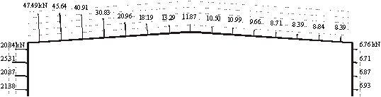
An example of the differences between the ASCE 7-93 loads and the loads based on the wind tunnel measurements is shown in Fig. 3. The assumed load, W_T, corresponds to the most unfavorable wind direction at a knee of frame 1 (wind parallel to the plane of the frame). Overall, W_T is considerably less unfavorable than the ASCE 7-93 load W_S, but there are exceptions which render the ASCE 7-based design inconsistent with respect to risk, as will be seen in Table 5.

For Frames 1 through 4, and for each of wind directions 0° to 120° at 5° intervals, Table 3 shows the peak knee-joint bending moments induced in the linear structure by external wind loads W_T due to the 50-yr wind speed specified in the ASCE 7-93 Standard. These moments include the effect of the time-invariant internal pressures. Also shown in Table 3 are the times at which those peak values occurred, in non-dimensional units k. The total length of the wind tunnel record (corresponding to a prototype time of about one hour) is k_max.t₁= 59.78 s, where t₁=1/400s is the time step of the wind tunnel time series, and the largest value of k is k_max=23912. The numbers in bold type indicate the frame with the largest knee-joint bending moment for each wind direction.

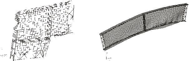
Figure 2.  Examples of local buckling failures (after [16])

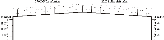
(a)

(b)

Figure 3.  (a) Wind forces W_S, specified by ASCE 7-93 Standard; (b) wind forces W_T, obtained from aerodynamic database for frame 1, wind direction normal to ridge [16]

Table 4 lists the nominal load factors l defining the ultimate capacities of Frame 1 for all load combinations corresponding to the wind load based on the aerodynamic database, W_T, and to the ASCE 7-93 Standard load, W_S. The comparison is made for the 90° direction, that is, the most unfavorable direction for this frame. It is seen that in this case the ASCE 7-93 load results in considerably lower l values – in more conservative designs – than the values based on the more realistic wind loading obtained from the aerodynamic database.

Table 5 lists calculated values of l for load cases 5 and 7 and the critical frames, corresponding to wind directions 0° to 120°. Also shown are values of l corresponding to the ASCE 7-93 loads. The ASCE 7–93 loads are conservative for Frames 1 and 2. However, for Frame 4, for directions 20° and 30° the l factors computed by using W_S are smaller than those computed by using W_T. In this and similar cases W_T induces moments at cross sections near the ridge and quarter-points of the rafter that in some instances are larger than those induced by the ASCE 7-93 loads. The ASCE 7 loads can thus be unsafe, in spite of the overall larger material consumption they entail, owing to the use of conservative values of l for most other cross sections. A modest strengthening with respect to the ASCE-based designs of cross sections with insufficient capacities would increase the safety of the structure. On the other hand, the amount of material can be reduced for cross sections and frames with excess capacity, without detriment to the safety of the structure. We note that current automated fabrication technologies allow such economical use of differentiated frame designs. 

Table 3.  Maximum moment at knee joint due to 50-yr wind loads W_T

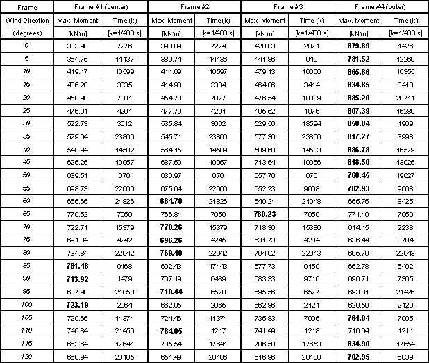
Table 4.  Nominal load factors corresponding to ultimate strengths of frame 1 for seven load cases 

Table 5.  Ultimate strengths and nominal load factors for various wind directions
(load cases 5 and 7)

* Ultimate strength of frames under wind loading obtained from ASCE 7-93 (see Table 3).

3.3       Purlins

Analyses similar to those reported in Section 3.2 for the interior frames were performed for purlins of the same building (see Section 3.1). Selected results are summarized in this section for Z-shaped purlins designed by MBMA/CECO. The purlins are continuous over four spans and have 45° braces at the end-span only. Grade 55 steel is used, and the wind loads, W_S, are based on ASCE 7-93 specifications. For the MBMA/CECO design the factor l under gravity load (loading Case 8 – see Section 3.1) is 1.58. For load cases 6 and 7 (see Section 3.1) failure involves buckling of the purlin section at the bottom flange-web junction after large twisting deformation near the center of the end span. For some wind directions the factors l are low (e.g., for Case 7, direction 80°, l=0.91), whereas for some other directions they can be quite high (e.g., Case 7, direction 130°, l=2.56). A comprehensive report on this investigation is being prepared by S. Jang and L.-W. Lu.

4.         Database-Assisted, Reliability-Based Design

4.1       Outstanding Codification Issues

The estimation of wind loads and of the reliability of wind-excited structures has been investigated extensively during the last few decades. However, the following issues still need to be addressed by code writers:

1.      According to the methods used by Ellingwood et al. [15] estimates of safety indices for structures designed in accordance with the ASCE 7 Standard are considerably lower for wind loading than for gravity loading. There appears to be no evidence supporting results obtained by those methods, particularly for wind-load resisting systems.

2.      In the ASCE 7 Standard, load factors are calculated as the ratio between point estimates of 500-yr and 50-yr wind loads, without regard for knowledge uncertainties. Wind load factors so calculated are referred to in this paper as nominal wind load factors, in contradistinction to wind load factors properly so called, which are calculated (e.g., in [15]) by accounting for at least some knowledge uncertainties. For example, the ASCE 7 Standard is based on the incorrect assumption that sampling errors are negligible if the size of the hurricane wind speed data sample generated by Monte Carlo simulation is large (i.e., of the order of 10,000). However, this assumption does not account for the significant sampling errors in the estimation of hurricane wind speeds that are due to the relatively small size (e.g., about 50 for any given location) of the climatological data sets on which the hurricane simulations are based [11].

3.      In the ASCE 7-98 Standard and its predecessors peak wind effects are based on records taken in the wind tunnel over periods equivalent to one-hour in full scale. Wind tunnel operators sometimes specify peaks based on records longer than one hour – in some instances as long as tens of hours. However, record lengths of one hour or even less, say 30 min, can be sufficient for codification purposes, provided that the associated uncertainties in the estimation of the peaks, as well as the other relevant variabilities and knowledge uncertainties, are taken into account within a structural reliability framework.

4.      Wind directionality effects in low-rise buildings are accounted for in the ASCE 7 Standard via multiplication by a reduction factor equal to 0.85, applicable to both main wind-load resisting systems and components. Recent research shows that this approach is, in general, not adequate. In particular, wind effects reductions due to wind directionality effects are less significant as the mean recurrence interval of the wind effects increases, rendering the use of the 0.85 factor potentially unsafe, particularly for wind-load resisting systems.

5.      Estimates of probability distributions of wind effects are useful for ensuring risk-consistency in standard provisions for wind loads. However, currently there are no practical and routine procedures for the estimation of probabilities of exceedance of specified wind effects in any one year. DAD used in conjunction with structural reliability methods can result in the development of such procedures, as is shown subsequently.

Some of these topics were dealt with in [18]. In this section we report more recent progress toward resolving the issues just listed, and describe the physical, probabilistic, and statistical ingredients used to develop reliability-based provisions. We also present the outline of procedures recently developed at NIST for the estimation of wind load factors and probabilities of exceedance of wind effects in one year.

4.2       Wind Effect Model

We denote by F_pk(t,N) the peak wind load effect with an N-year nominal mean recurrence interval, occurring in the prototype subjected to the action of a storm with duration t. The time interval t can be, say, 20 min, 30 min, 1 hour, or longer, and the storm is assumed to induce wind loads that may be assumed to be a statistically stationary process. Thunderstorm wind effects may be considered provided that stationary records yielding comparable peak wind effects are used in the calculations. The nominal mean recurrence interval can be, say, 50 years, 500 years, or 10,000 years. We use the model

     F_pk(t,N) = ½ rC_pk(t)abcV²(t,H_aero,z_o,N)                                                                                        (6)

where r is the air density, for which no uncertainty need to be considered; C_pk(t) is the random peak factor for the fluctuating wind effect (e.g., bending moment) induced by the storm, and is a measure of the largest peak wind effect occurring during time t. V(t, H_aero, z_o, N) is the wind speed at reference height H_aero, averaged over the time interval t. The nominal mean recurrence interval of the wind speed is N, in years, and the roughness of the terrain that characterizes the site upwind of the building is z_o. H_aero is commonly chosen to be the height of the top of the building or the eave height. The quantities a, b, c are random variables associated with imperfect knowledge (“epistemic” or knowledge uncertainties), as opposed to randomness inherent in a variable (“aleatory uncertainties”). For example, the terrain roughness is usually known with some uncertainty, whereas the wind speed is an inherently random variable. Unless otherwise indicated, all uncertainty variables, including a, b, c will be assumed to have normal distributions with mean unity. The variates a, b, c are defined as follows. The variate a reflects aerodynamic errors inherent in the wind tunnel being used, since results of wind tunnel tests may depend upon the test facility. The variate b reflects aerodynamic errors due to (a) the use of wind tunnel rather than full-scale measurements, and (b) imperfect wind tunnel to full-scale data calibration. The variate c reflects errors in the transformation of aerodynamic effects into stresses or other structural effects.

If wind directionality effects are taken into account, V(t,H_aero,z_o,N) is replaced in Eq. 6 by an equivalent speed denoted by V_eq(t,H_aero,z_o,N) determined as shown in Section 5.5. Unless specifically needed we omit in the subsequent developments the subscript “eq,” since reliability calculations involving equivalent wind speeds are similar in form to those involving wind speeds estimated without regard for directionality.

4.3       Wind Speed Model

The wind speed is estimated by using:

·        Measured or simulated wind speed data at the standard meteorological elevation H_met (e.g., 10 m above ground) in open terrain with standard roughness z_o1 (e.g., z_o1 = 0.05 m). The averaging time T for the wind speed data varies. In the ASCE 7-98 Standard the interval T = 3 s is used. Simulated hurricane wind speed data available in NIST public files and based on [6] are averaged over one minute. From these observed or simulated wind speed data, point estimates can be made of wind speed data with various mean recurrence intervals.

·        Conversion factors r that account for wind speed averaging time. To obtain wind speeds averaged over time t, wind speeds averaged over time T are multiplied by the factor r(T, t). While, like all our uncertainty variables, we assume r to be normally distributed, its mean is not unity. Rather, the means of the variable r(T, t) are obtained from ASCE 7-98 [14, p. 140] as functions of T and t (see also [19]).

·         Factors that convert wind speeds averaged over time t over open terrain with roughness z_o1 at the standard meteorological elevation H_met to wind speeds averaged over time t at the aerodynamic reference elevation H_aero over the terrain with roughness z_o upwind of the building. These factors are yielded by the logarithmic law and the relation between wind speeds in different roughness regimes [19, pp. 42, 48], and are functions of z_o1 and z_o. (Effects of terrain fetch that may be insufficient for the full development of the boundary layer, or of escarpments/hills, are not considered here but may be introduced in the model.) We denote by u and s the random variables, assumed to have mean unity and truncated normal distributions that reflect the uncertainties with respect to the actual values of z_o1 and z_o. The following approximate expression is obtained:

                                                (7)

where d=0.0706 may be assumed to have negligible variability. The factor u_H in Eq. 7 reflects the uncertainty with respect to the applicability of this model to hurricane wind speeds, which differ to some extent from extratropical wind speeds. For extratropical storm winds the factor u_H is, by definition, unity; for hurricane wind speeds its mean and coefficient of variation are assumed to be unity and 0.05, respectively. The variable q accounts for observation errors, and has a truncated normal distribution with mean unity.

It is assumed that the quantities involved in the calculation of wind effects are estimated on the basis of sound information, for example, information obtained from wind tunnels that meet standard performance criteria and are calibrated against dependable full-scale results; or information from certified weather stations. We do not consider gross errors or errors inherent in information based on substandard sources.

4.4       Estimation of Wind Speeds Without Regard for Directionality

Denote the mean and the standard deviation of the sample of extreme wind speeds by E(X) and s(X), respectively. Expressions for the Extreme Value Type I (EV I, or Gumbel) distribution and its inverse (the variate corresponding to a mean recurrence interval N in years) and the EV III (or reverse Weibull) distribution are given, e.g., in [11]. If very large time series of extreme wind speeds estimated without regard for direction are available, then extreme wind speeds with various mean recurrence intervals may be estimated simply and directly without fitting a distribution to the data – see [7] for details. This alternative has been used in some instances for hurricane wind speeds.

4.5       Equivalent Wind Speed Reflecting Effect of Wind Directionality

If extreme wind rosettes are available – as is the case for simulated hurricane wind speed data – equivalent hurricane wind speeds are calculated as shown in [7]. For the sake of clarity we consider a deliberately simple illustrative example of the approach presented in [7]. In this example aerodynamic data are available for m = 2 directions (say, 0° and 180°), extreme wind climatological data are available for n = 2 directions, and the number of simulated extreme hurricane wind speed rosettes is k = 3. (In practical applications one would commonly have
m = 72, n = 8 or 16, and k = 999 or larger.)

We denote the bending moment induced in cross section i of frame j by a wind load with mean hourly speed 1 m/s blowing from direction 2 by m_ij(2). These quantities may be viewed as directional influence factors (DIFs). The DIF m_ij(2) times the square of the wind speed blowing from direction 2 yields the moment M_ij(2) induced by that wind speed in cross section i of frame j. DIF’s for the cross section and frame of interest are given in Table 6. Three cases are of interest in engineering and codification practice. The calculations involved in the three cases are based on the information of Tables 6 and 7.

Table 6. Moment DIF’s (in kN^.m) 

Table 7. Wind speed rosettes (in m/s) 

Case 1. Circular wind rosette. Assume that the wind rosettes of the extreme wind speeds are circular with radii max_n[V(n,k)] (k = 1,2,3). Then the time series of the largest moments are max_n [M_ij(n,k)] = {51² x 100 = 260100, 46² x 100 = 211600, 49² x 100 = 240100} kN^.m, i.e. the extreme wind effect is equal to the square of the specified wind speed times the largest m_ij. The largest calculated moment in the three storm events is 260100 kN^.m. The second largest in the three storm events is 240100 kN^.m.

Case 2. Building with known orientation. Consider the case of a building whose axis normal to the plane of the frames is parallel to the north direction (i.e., has an orientation defined by a 0° angle). From Tables 6 and 7 the results for the moments M_ij(n,k) at cross section i of frame j are obtained and presented in Table 8.

The largest calculated moment in the three storm events is 230400 kN^.m, that is, significantly less than the value 260100 kN^.m calculated by disregarding the effect of the climatological directionality. In this case the ratio between the moment calculated by taking into account both the aerodynamic and climatological dependence upon direction and the moment calculated by disregarding the effect of the climatological wind direction is K_d = 230400/260100 = 0.89. For the second largest moments in the three storms the ratio is K_d = 211600/240100 = 0.88. Calculations effected for cases of practical interest have shown that in general the factor K_d is an increasing function of mean recurrence interval [7] and approaches unity for the large mean recurrence intervals associated with ultimate limit states. In contrast the wind effects calculated by the ASCE Standard as in Case 1 above are multiplied in that Standard by a blanket factor K_d = 0.85. We note that the closeness to this value of the 0.88 and 0.89 values calculated earlier is coincidental.

Table 8. M_ij(n,k) (in kN^.m) 

Case 3. Buildings with unknown orientation. This case corresponds to the reality of most designs based on code provisions for wind loads. The analysis should be performed for all possible orientations of the building (in our deliberately simple case 0° and 180°). The M_ij value of interest is the largest of the values obtained for the various building orientations. If the distribution of orientations at a particular geographical location is known it is possible to obtain statistics of the moment of interest, which may be used along with the other relevant statistics within the framework of a reliability analysis. A similar analysis may be warranted for loss estimation purposes.

The time series of the equivalent wind speeds V_eq(k) is defined, to within a constant, as the time series of the square roots of the quantities max_n [M_ij(n,k)]. For details see [7]. Note that in the procedures presented here it was assumed that the terrain roughness is independent of direction. The procedure can be modified to accommodate the case where this assumption does not apply.

4.6       Sampling Errors in Extreme Speeds Estimation

The mean E(X) and the standard deviation s(X) must be estimated from an n-year record {x₁,x₂,…,x_n} of the extreme wind speeds using standard expressions. Expressions for the sampling errors in the estimation of the wind speed with average return period N years are given in [11]. For hurricane-prone regions the estimates of extreme wind speeds are obtained by using the peaks over threshold approach. Sampling errors are estimated on the basis of the number of data that exceed the respective thresholds. However, the data themselves are obtained by Monte Carlo simulation from information on relevant climatological parameters: pressure differences between the edge and the center of the hurricane, radius of largest hurricane wind speeds, and the translation velocity of the hurricane. This climatological information is based on records of about 100-year length, corresponding to a total number of hurricanes at a particular location of about 50 (depending upon geographical location). Therefore the climatological information on which the simulated hurricane data is based is itself subjected to sampling errors. The effect of these sampling errors on the estimated extreme wind speeds regardless of direction based on simulated data was studied in [20]. For example, the coefficients of variation of the sampling errors in the estimation of the 100-yr and 10,000-yr wind speeds are typically of the order of 0.10 and 0.20, respectively. The total sampling error depends upon the threshold. Its variance is equal to the sum of the variance associated with the size of the simulated data sample used in the estimates (this variance is usually negligible) and the variance associated with climatological parameter uncertainties. Sampling error estimates for calculations that account for wind directionality are similar to those performed for the case of wind speeds estimated without regard for direction, except that they are based on equivalent wind speeds estimated as shown in [7].

4.7       Peak Factors

The peak factors C_pk are in general non-Gaussian. A numerical procedure for estimating the probability distribution of the peak is incorporated in the software for estimating peak wind effects [10]. C_pk will depend on the particular sample considered in the analysis and on its size. Sampling errors in the estimation of C_pk are obtained as shown in [12]. In a simpler but less accurate estimate the peak factors are taken to be equal to their observed values.

4.8       Wind Load Factors

All results in this section were obtained by Monte Carlo simulation, the number of samples in each simulation being n_s = 2000 [11]. We consider separately the cases of non-hurricane and hurricane winds.

Regions Not Subjected to Hurricane Winds. The wind load factor is defined in the ASCE 7-98 Standard as the square of the ratio between the point estimate (the 50 percentile) of the 500-yr wind speed and the point estimate of the 50-yr wind speed. Both estimates are based on the assumption that the extreme wind speeds are best fitted by the Extreme Value Type I distribution. The ASCE 7-98 Standard further specifies that the structural member experience the state associated with strength design and defined as 50-yr wind effect times the ASCE 7 wind load factor [14, p. 114].

As was mentioned earlier, the ASCE 7 definition does not account for knowledge uncertainties. These uncertainties are considerable, and disregarding them may result in unrealistic estimates. It may be argued that using an infinitely-tailed probabilistic model for the wind speeds, when in fact wind speeds are more realistically described by a finite-tailed model, compensates for the failure to account for errors and uncertainties. However, this is in general not the case. For this reason Ellingwood et al. [15, p. 115] specifically accounted for errors and uncertainties in their estimates of safety indices.

We therefore define wind load factor as follows. As in the ASCE 7 Standard, we assume that the wind effect for strength design (corresponding., e.g., to the attainment of the yield stress by a cross section’s most stressed fiber) is induced by a wind speed with a 500-yr mean recurrence interval (ASCE 7-98 Standard Commentary, p. 114). However, we do not consider the point estimate of the 500-yr wind effect, since there is a chance of approximately 50 percent that the true 500-yr wind effect would be larger than the point estimate. Noting that in the development work for the ANSI A58 Standard (the predecessor of the ASCE 7 Standard) Ellingwood et al. [15] considered the 90 percentile for the estimates of 50-yr wind effects, we choose to define the wind load factor as follows:

     LF = F_pk(N=500-yr, 0.9) / F_pk(N=50-yr, 0.5)                                                                              (8)

where 0.9 and 0.5 denote the 0.9 percentage point and the 0.5 percentage point, respectively. In other words, multiplying the point estimate of the 50-yr wind effect by the estimated load factor LF yields the 90 percentile of the 500-yr wind effect. This definition is reasonable and useful for our purposes; we do not view it as normative, however, and consensus might be reached on alternative definitions. The load factor estimates depend upon the probability distribution of the extreme wind speeds assumed in their estimation. The Type I distribution of the largest values was until relatively recently universally believed to be a correct probabilistic model of the extreme wind speeds. A significant body of research conducted following the development in the 1970’s of modern extreme value theory and approaches, including peak-over-threshold methods, strongly suggests that extreme wind speeds are better fitted by Type III distributions of the largest values which, unlike the Type I distribution, have bounded upper tails [21-27]. We performed Monte Carlo simulations for estimating load factors LF by using first the Gumbel distribution and then the reverse Weibull distribution, all other assumptions and parameters being the same. Sampling errors in the estimation of the extreme wind speeds, and peak values and sampling errors in their estimation, were obtained as indicated in Section 4.6. The basic set of parameter values used in the calculations is listed in Table 9.

Table 9. Basic set of means and standard deviations of the uncertainty parameters, assumed to be normally distributed

In addition, it was assumed that the roughness lengths are z_o = 1.00 m and z_o1 = 0.07 m. We note that recent work [28] considers the more realistic case c.o.v.(s) = c.o.v.(u) = 0.3, with the values z_o = 0.40 m and z_o1 = 0.05 m.

We now discuss briefly the influence on the results of the calculations of the assumed probabilities of the extreme wind speeds. The results showed that estimated load factors are significantly larger if an infinite-tailed model (EV I), rather than a finite-tailed model (EV III), is used to describe the distribution of the largest wind speeds. For example, for the parameters of Table 9, if the sample coefficient of variation of the extreme wind speed data is c.o.v. = 0.15, then LF = 1.55 under the assumption that the reverse Weibull distribution with tail length parameter c = - 0.2 is valid, and LF = 1.90 under the assumption that the Extreme Value Type I distribution is valid. (The tail length parameter c = -0.2, while not universally valid, is usually a reasonably conservative approximation for most stations – see [22]. These results are typical.

Under the assumption that the extreme wind speeds have a reverse Weibull distribution it follows from our results that load factors based on a Gumbel distribution are significantly overestimated. This view is consistent with experience embodied in wind load factor values incorporated in standards. It thus appears that the reason for the low safety index estimates for wind loads obtained by the procedure used in [15] is the use in that procedure of the assumption that extreme wind speeds are best fitted by the EV I distribution. Using this assumption for the estimation of wind speeds with relatively short mean recurrence intervals (50 years, say) is, by and large, acceptable. The assumption becomes onerous if it is used for long mean recurrence intervals, such as those associated with strength design or ultimate structural capacity.

After multiplication by the wind direction reduction factor, assumed in the ASCE 7 Standard to be 0.85, the load factor specified in the ASCE 7-95 Standard for non-hurricane winds is 1.3. Before reduction, the load factor is 1.3/0.85 = 1.53 (i.e., close to our calculated value corresponding to the reverse Weibull assumption, LF = 1.55). The ASCE 7-95 value of the load factor was based on engineering judgment and experience, rather than on the safety index calculations reported in [15]. We note the agreement of our estimated value with the ASCE 7-95 value. We also note that the value 1.53 was augmented in the ASCE 7-98 Standard (p. 4, Section 2.3.2) to 1.36/ 0.85=1.6 (rather than being 1.5, as is indicated erroneously in the Commentary to the Standard, see ASCE 7-98, p. 114). This augmented value is still approximately consistent with our calculated value LF = 1.55. The reason for this consistency lies in our choice of uncertainty parameters, which we believe is reasonable. Should it be considered necessary to use different uncertainty parameters, the estimated value of the load factor would change to some extent.

Regions Subjected to Hurricane Winds. We performed simulations with the basic set of uncertainty parameters of Table 1, using the 999 simulated T = 1-min hurricane wind speeds for a northwestern Florida coast location. The speeds are part of the hurricane wind speed database developed by Batts et al. [6]. Hurricane wind speeds are best fitted by reverse Weibull distributions for which it is reasonable to assume a tail-length parameter c = -0.2 [23]. Estimates of coastal hurricane wind speeds with mean recurrence intervals of 50 to 2,000 years based on this assumption are consistent with estimates obtained independently by other authors [29]. In our simulations the distribution fitted to the extreme wind speeds was reverse Weibull with tail length parameter c = -0.20. The distribution parameters were found by using the peaks over threshold method. Sampling errors in the estimation of the extreme wind speeds, and peak values and sampling errors in their estimation, were estimated as indicated earlier in the paper. The basic set of parameter values used in the calculations is listed in Table 9.

Our calculations yielded the hurricane wind load factor LF = 2.14. This result should be compared with the load factor LF = 1.55 obtained, with the same set of uncertainty parameters, for extratropical wind speeds with coefficient of variation c.o.v = 0.15, assumed to be best fitted by the reverse Weibull distribution with c = -0.20. The result that load factors for hurricane-prone regions are larger than for non-hurricane regions is not new [25]. However, we believe that the methodology presented here allows a more realistic estimation of the load factors, insofar as we take into account the various uncertainties discussed in this section. Numerous sensitivity studies reported in [11] confirm the reasonableness of our results.

4.9       Influence of Length of the Time Series of Wind Pressure Coefficients Measured in the Wind Tunnel

Estimates of wind effects depend upon the length t of the time series of the pressures recorded in the wind tunnel. This dependence is of interest insofar as unduly long recording periods might create data storage problems for aerodynamic databases on buildings with a large number of pressure taps. On the other hand, a too short length t would cause unacceptable sampling errors in the estimation of extreme wind effects.

Simulations for three cases: t = 1 hr, t = 30 min, and t = 20 min are reported in [12]. Typical sampling errors in the estimation of peak wind effects corresponding to 1-hr records have coefficients of variation of about 5 %. Their consideration in reliability calculations increases requisite safety margins by about 3 %. If the records being considered are 30-min long the increase is about 5 %. Therefore for peaks typical of internal forces in frames of low-rise buildings 30-min records appear to be adequate for codification purposes.

4.10     Probability Distributions of Wind Effects

The procedure described in this section can be used to estimate probability distributions of wind effects. The peak wind of interest is expressed in Eq. 6 as a function of mean recurrence interval N = 1/(1 – p), where p is the probability of exceedance of the wind effect in any one year. Recall that the wind effect is a function of stochastic variables with specified distributions, including variables reflecting knowledge uncertainties. For any specified p (or N) the wind effect of interest is obtained by applying the total probability theorem to the expression of the wind effect, that is, by integrating the expression of the wind effect over the set on which the stochastic variables are defined. User-friendly software that yields estimates of the requisite wind effects corresponding to various probabilities of exceedance, p, is currently being developed for use in conjunction with database-assisted definitions of wind effects.

5.           Archiving Aerodynamic Databases. Database-Assisted Design and Computational Fluid Dynamics

UWO, in collaboration with NIST, TTU, and Purdue University, is developing a protocol for archiving aerodynamic databases that will make it possible to use DAD software with databases from all sources that will adopt that protocol.

We feel it is useful to mention that DAD is ideally suited for use with time histories obtained by Computational Fluid Dynamics (CFD) techniques. Such techniques are not yet developed to allow their use at the present time. However, it is anticipated that this will change in the not too distant future. When CFD will be used in conjunction with CFD design, uncertainties associated with terrain roughness definition around structures to be designed in built-up terrain will decrease significantly. It may be expected that the definition of the wind loads will be achievable routinely in the design office and will no longer need to be based on wind tunnel testing to the same extent that it is today.

6.         Conclusions

Significant improvements in main wind-load resisting system and component design can be achieved by using database-assisted design (DAD) methods and associated structural reliability tools, thus accounting realistically for the complexity of the wind loading as well as for the stochasticity and knowledge uncertainties affecting wind effects calculations. In this paper we showed that DAD can be used to obtain realistic estimates of nominal wind load factors and of failure probabilities associated with ultimate limit states due to local or global buckling failure and, in the future, to other types of nonlinear behavior. In particular, we showed that the ASCE 7 Standard assumption that aerodynamic pressure coefficients for low-rise buildings are independent of terrain roughness is not correct. We also showed that the use of ASCE 7 wind loading provisions can result in large errors – up to 60 % -- in the estimation of wind effects. We presented results demonstrating that DAD can be used in conjunction with nonlinear analysis methods to define realistic ultimate limit states and the corresponding wind loads and nominal wind load factors. To our knowledge this is the first set of results obtained in wind engineering that accounts for both the actual distribution of the wind loads and the ultimate limit states of frames and components susceptible to buckling. The approach used to obtain such results represents a major step forward with respect to conventional code approaches, where ultimate limit states are not considered explicitly.

Acknowledgment

An expanded version of this paper was presented at the A.G. Davenport Symposium, London, Ontario, June 2002.

References

[1]  Fleming, R., 1915, Wind Stresses, Engineering News, New York.

[2] Flachsbart, O., 1932, Ergebnisse der Aerodynamischen Versuchanstalt zu Göttingen, IV Lieferung, L. Prandtl and A. Betz (eds.), Verlag von Oldenburg, Münich and Berlin.

[3] Davenport, A.G., Surry, D., and Stathopoulos, T., 1977, Wind Loads on Low Rise Buildings: Final Report of Phases I and II, Parts 1 and 2, BLWT-SS8-1977, London, Ontario, Canada.

[4] Lin, J., and D. Surry, 1997, Simultaneous time series of pressures on the envelope of two large low-rise buildings, BLWT-SS7-1997, Boundary Layer Wind Tunnel Laboratory, University of Western Ontario, London, Ontario, Canada.

[5] TTU/NIST Collaborative Study, 2001, Ho, E. (Research Director), BWLT File T019, London, Ontario, Canada.

[6] Batts, M.E., Russell, L.R., and Simiu, E., 1980, “Hurricane Wind Speeds in the United States,” J. Struct. Div., ASCE 106 2001-2015.

[7] Rigato, A., Chang, P., and Simiu, E., 2001, “Database-Assisted Design, Standardization, and Wind Direction Effects,” J. Struct. Eng., 127 855-860.

[8] Whalen, T.M., Shah, V., and Yang, J.-S., 2000, “A Pilot Project for Computer-Based Design of Low-Rise Buildings for Wind Loads – The WiLDE-LRS User’s Manual, NIST Contractor Report 00-802, National institute of Standards and Technology, Gaithersburg, MD, USA.

[9] Gioffrè, M., Gusella, V., and Grigoriu, M., 2001, “Non-Gaussian Wind Pressure on Prismatic Buildings II: Numerical Simulation,” J. Struct. Eng., 127 990-995.

[10] Sadek, F., and Simiu, E., 2002, “Peak Non-Gaussian Wind Effects for Database-Assisted Low-Rise Building Design,” J. Eng. Mech., 128 530-539.

[11] Minciarelli, F., Gioffrè, M., Grigoriu, M., and Simiu, E., 2001, “Estimates of Extreme Wind Effects and Wind Load Factors: Influence of Knowledge Uncertainties,” Prob. Eng. Mech., 16- 331-340.

[12] Sadek, F., Diniz, S., Kasperski, M., Gioffre, M., and Simiu, E., 2002 “Sampling Errors in the Estimation of Peak Wind-Induced Internal Forces in Low-Rise Structures,” J. Eng. Mech. (submitted).

[13] ASCE 7-93 Standard Minimum Design Loads for Buildings and Other Structures, 1999, American Society of Civil Engineers, New York, NY, 1994.

[14] ASCE 7-98 Standard Minimum Design Loads for Buildings and Other Structures, American Society of Civil Engineers, Reston, VA, 1999.

[15] Ellingwood, B. R., Galambos, T., McGregor, J., and Cornell C. A., 1980, Development of a Probability Based Load Criterion for American National Standard A58, NBS Special Publication 577, National Bureau of Standards, Washington, D.C.

[16] Jang, S., Lu, L.-W., Sadek, F., and Simiu, E., 2002, Database-Assisted Wind Load Capacity Estimates for Low-Rise Steel Frames,” J. Struct. Eng. (in press).

[17] ABACUS Standard, 1999, Hibbit, Karlsson and Sorensen, Inc., Providence, Rhode Island.

[18] Ellingwood, B.R., and Tekie, P.B., 1999, “Wind Load Statistics for Probability-Based Structural Design,” J. Struct. Eng .125 453-463.

[19] Simiu, E., and Scanlan, R.H., 1996, Wind Effects on Structures, 3^rd ed., Wiley-Interscience, New York.

[20] Batts, M.E., Cordes, M.R., and Simiu, E., 1980, “Sampling Errors in Estimation of Extreme Hurricane Winds,” J. Struct. Div., ASCE 106 2111-2115.

[21] Simiu, E., and Heckert, N.A., 1996, “Extreme Wind Distribution Tails: A Peaks-Over-Threshold Approach,” J. Struct. Eng 122 539-547.

[22] Walshaw, D., 1994, “Getting the most out of your extreme wind data,” Journal of Research of the National Institute of Standards and Technology 99 399-411.

[23] Heckert,, N.A., Simiu, E., and Whalen, T.M., “Estimates of Hurricane Wind Speeds by ‘Peaks Over Threshold’ Method,” J. Struct. Eng., 124 445-449.

[24] Holmes, J.D., and Moriarty, W.W., 1999, “Application of the Generalized Pareto Distribution to Extreme Value Analysis in Wind Engineering,” J. Wind Eng. Ind. Aerodyn., 83 1-10.

[25] Whalen, T., and Simiu, E., 1988, “Assessment of Wind Load Factors for Hurricane-Prone Regions,” Structural Safety 20 271-281.

[26] Simiu, E., Heckert, N.J., Filliben, J.J., and Johnson, S.K., 2001, “Extreme Wind Load Estimates Based on the Gumbel Distribution of Dynamic Pressures: An Assessment,” Struct. Safety, 23 221-229.

[27] Galambos, J., and Macri, N., 1999, “Classical Extreme Value Model and Prediction of Extreme Winds,” J. Struct. Eng., 125 792-794. Discussions by E. Simiu and J.A. Lechner, and by J.D. Holmes, and Closure, J. Struct. Eng., 128 271-275.

[28] Diniz, S.M.C., Sadek, F., Simiu, E., 2002, “Wind Speed Estimation Uncertainties: Effects of Climatological and Micrometeorological Parameters,” in preparation.

[29] Vickery, P.J., and Twisdale, L.A., 1995, “Prediction of Hurricane Wind Speeds in the U.S.,” J. Struct. Eng., 121 1691-1699.