 (1)
(1)
Euro-SiBRAM’2002 Prague, June 24 to 26, 2002, Czech Republic
To the Discussion on the Earthquake Loading in SiBRA
Prof. Ondřej Fischer
Institute of Theoretical and Applied Mechanics, Academy of Sciences of the Czech Republic
Prosecká 76, 19000 Praha 9
Abstract
The impossibility of using the Arbitrary Point in Time-approach for the probability of occurence (for the construction of a regular histogram, used for ordinary loadings in static analysis) of earthquake loading is shown by an attempt to construct such a histogram based on the checked probabilities of real earthquakes.
1. Solution to the earthquake response on structures
In principle, three approaches can be distinguished for the solution of the response of structures to earthquake loadings (to the design of structures for earthquake resistance), viz:
aa) classical, quasi static approach (most codes, incl. Eurocode 8): The effect of earthquakes is equal to the effect of equivalent seismic forces, acting as static loading.
ab) dynamic solution of the response of the structure to the seismic excitation, given as a time function representing usually the real or artificial accelerogram a(t) (most codes, incl. Eurocode 8 for important structures)
ac) stochastic – the set of real accelerograms in the zone under consideration is treated as a non-stationary random process and characterized by some statistical parameters. The statistical parameters (mean values, dispersals) of the response of the structure are solved using the methods of stochastic mechanics (see Náprstek-Fischer 2002).
Note: All approaches are burdened with the lack of real input data – here, in the first row, the parameters of future earthquakes.
Probabilistic character of the problem of earthquake resistant structures can be seen in three aspects:
ba) definition of the earthquake to which the structure may resist (ground acceleration, time-course of the seismic motion or its statistical characteristics, all given by histograms). The design earthquake should be known from codes or from the geophysicist’s expertise, similarly as all other common loadings of any other structure
bb) probability of occurence of the disastrous earthquakes, something like the time-duration curves in standard SiBRA solution (it is a problem – see later)
bc) parameters of the structure used for the solution of its safety (dimensions, material characteristics, real behaviour of supports etc, again given by histograms, similarly as in a static structural design).
For the following considerations only the most simple one, namely the quasi static approach (classed above as aa), is used. For the other ones, mutatis mutandis the same can be said.
2. Seismic forces
Seismic force, acting as a static horizontal force which substitutes the maximum effect of an earthquake, is in the majority of codes in principle defined as
(1)
![]()
where
![]() -
design ground acceleration
-
design ground acceleration
q - behaviour (ductility) factor
m - total mass of the building
T1 - 1st natural period
Sd(T) - design spectrum (dynamic amplification function see Fig.1)
Fig. 1 Design spectrum vs. natural period
3. Probability of occurence of an earthquake
According to the codes the intensity of the design earthquake is usually given by the return period of the event, which e.g. in Eurocode 8 is 475 years. This theoretically means that, if the duration of an earthquake is 1 minute, or, including 4 aftershocks of the same intensity, 5 min., the probability that the earthquake loading is being applied, is
(2)
Pr =
![]() 2.10-8
2.10-8
and this should also be
the probability of occurence of the design ground acceleration
![]() and
of the loading by the seismic force Fs,b,max
(1) given above.
and
of the loading by the seismic force Fs,b,max
(1) given above.
To come slightly nearer to the reality lets suppose that the earthquake can come (that the random event with the return period of 475 years can come) at any moment during the life-time of the structure, e.g. during 50 years (cf. the “Arbitrary Point in Time”-approach in Václavek 2002). Then the probability of occurence of the seismic loading by the force (1) Fs,b,max is
(3)
Pr =
![]() 1.90.10-7
1.90.10-7
Lets try now to calculate the probability of occurence of smaller earthquakes, and lets be known that the seismic activity of the magnitudo smaller by 2 can be in the zone observed for together 1 hour per year. As the magnitudo is a logarithmic function of the energy of vibrations, the seismic force corresponding to this smaller shaking is Fs,b,-2 = 0.01 Fs,b,max .
One other aspect to be mentioned is the behaviour factor q in (1). It is in most cases introduced as 4 and – schematically spoken – its scope is the reduction of the seismic force due to the fact that the strong earthquakes occur very rarely and that the use of plastic reserve in the design can be admitted. In the case of 1 hour earthquakes such a reduction cannot be used, and the force corresponding to the small earthquakes is to be considered without the reduction by q , i.e. 4 times larger, viz.
(4) Fs,b,-2 = 0.04 Fs,b,max
The probability of occurence of weaker, one hour lasting shaking per year is
(5)
Pr =
![]() 1.1415.10-4
= 0.00011415
1.1415.10-4
= 0.00011415
In order to construct a histogram from these values lets suppose that the seismic force was determined with the accuracy of 1% - in other words, the event occuring with the probability calculated in (3) means that the calculated value of the seismic force lies in the interval of the width ΔFs = 0.01 Fs,b,max, i. e. that it holds 0.99 Fs,b,max < Fs,b < Fs,b,max.
Using this presupposition, the ordinates of seismic force histogram f(Fs,b) corresponding to the probabilities (3) and (5), will be:
f(Fs,b,max) = 1.90.10-7 : 0.01 = 1.90.10-5 ; f(0.04 Fs,b,max) = 0.00011415 : 0.01 = 0.011415
Between these two values, the histogram of the seismic forces corresponding to earthquakes of intermediate intensities is supposed to be linear (Fig. 2). From this histograms it can be drawn out that the entire probability of the seismic force in the interval (0.04 ~ 1.0) Fs,b,max is
Pr [0.04 Fs,b,max < Fs,b < Fs,b,max ] = (1.90.10-5 + 1.1415.10-2) : 2 ∙ 0.96 = 5.4883.10-3 ,
and the probability of negligible seismic force (smaller than 0.04 Fs,b,max) is the complement to one, viz. 1 – 5.488.10-3 = 0.994512 . The ordinate of the histogram in the interval
f(0 < Fs,b < 0.04 Fs,b,max) = 0.994512 : 0.04 = 24.8628 .
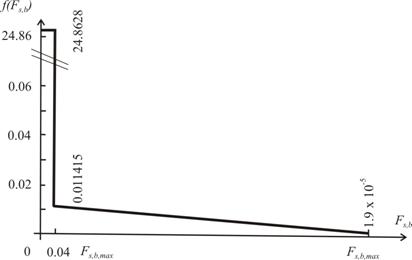
Fig. 2 Histogram of seismic forces based on return periods of earthquakes
4. Results
From the histogram (Fig. 2) and from the calculated probabilities it evidently results that the here demonstrated approach cannot be used for probability assessment of earthquake resistance of structures. The extremely small probability of earthquake occurence (0.5 %) means that only one from cca 200 simulation cycles would include (even the smallest) seismic loading, and that the maximum seismic force could occur once in 1 : 1.90.10-7 = 5.26 millions of cycles. Such values of probability, as well as the histogram taking into account the probability of earthquake-occurence during the life-time of the structure, are – in comparison with the probabilities of occurence of other loadings – irrelevant for the probability assessment of seismic resistance of structures. In fact, it should be supposed that the maximum design earthquake (given by geophysicists for the zone) can occur at any moment of the life of the structure, thus it has to be combined with all other loadings. In other words, the effort of using the probabilities based on return periods of earthquakes in Arbitrary Point in Time (APT) approach, which is used in case of combination of common load effect in SBRA method, is not appropriate, and Maximum Load Effect (MLE) of the earthquake (in the instant of an earthquake), together with the Arbitrary Point in Time (APT) combination of all other common load effects should be considered (see Vaclavek 2002).
One other important thing to be taken in mind is the quasistatic solution of earthquake effect by means of equivalent seismic forces, which is in principle incorrect and must be therefore “handled with care”. The calculated effect of seismic forces represents the structural response (stresses, displacements etc), which in reality corresponds to the amplitudes of vibrations, i.e. they may have both signs. This means that in one simulation cycle, the result of which should be the worst combination (sum) of different load effects, the effect of seismic forces should be considered twice with the signs + or -, and only the worse one is to be taken as the result of this cycle.
5. Conclusions
(i) The effort of expressing the probability of earthquake loading by means of its return period obtained from geophysicists is of no use, the earthquake should be expected to come at any moment, and should be combined with all realistic loadings. This means that the Arbitrary Point in Time (APT) approach is not appropriate, but the Maximum Load Effect (MLE) of the earthquake should be considered together with the APT combination of all other common load effects.
(ii) The
response to earthquake loading are vibrations, even if it has been
calculated as a response to static loading, and should be considered
as
![]() ,
i.e. should be both added or subtracted to the effects of all other
loads during one simulation cycle
,
i.e. should be both added or subtracted to the effects of all other
loads during one simulation cycle
Acknowledgement
The paper was prepared with the support of research projects No A2071002 and 103/01/1410 and this support has been gratefully acknowledged.
References
[1] Eurocode 8: Design of structures for earthquake resistance, Part 1: General rules, seismic actions and rules for buildings. Draft No 5, May 2002. CEN, Brussels
[2] Náprstek J., Fischer C. (2002): Non-stationary response of structures excited by random seismic processes with time variable frequency content. Jour. of Soil Dynamics and Earthquake Eng., July 2002, p. 21
[3] Marek P., Václavek L. (2002): Issues related to the probabilistic safety assessment of steel structures in the stability domain. In: Proc. 15th ASCE Engineering Mechanics Conf., June 2-5 2002, Columbia Univ, New York, NY-USA, 9 p.