Euro-SiBRAM’2002 Prague, June 24 to 26, 2002, Czech Republic

ASSIGNMENT

Reliability Assessment of an Unbraced Frame with Leaning Columns

Ing. Leo Václavek, PhD.

VŠB Technical University of Ostrava, 17.listopadu 15, 708 33 Ostrava-Poruba,Czech Republic

leo.vaclavek@vsb.cz

Prof. Ing. Pavel Marek, DrSc.

Institute of Theoretical and Applied Mechanics Academy of Sciences of Czech republic and Dept. of Civil.Eng. VŠB Technical University of Ostrava, Czech Republic

marekp@itam.cas.cz

ATTENTION: PLEASE  READ ASSIGNMENT

In order to start discussion on selected problems solved using the simulation-based reliability assessment method, and to allow for comparing compare different approaches, the Organization Committee of the Colloquium invites you to take part in following study.

The assignment (safety assessment of a planar frame exposed to load combination) is specified on the following pages. Following strictly this assignment, please determine the probability of failure of the steel frame (refer to the carrying capacity of the cross section marked X-X - see fixed end of the shorter column). The probability of failure should refer to the combination of the bending moment M and axial force A in x-x cross section.

Your solution, together with all other submitted solutions, will be considered for publishing in the second edition of the textbook "Probabilistic Assessment of Structures using Monte Carlo simulation. Basics, Exercises, Software" (Published by ITAM Academy of Sciences of Czech Republic, Prague) in 2003. If you are interested in participating, please follow instructions regarding typesetting, formatting, etc. given on web site www.itam.cas.cz/sbra/format.html (see "Second edition of TERECO book") and submit your solution by e-mail before March 20, 2003 to the address indicated on the web page.

The Organizing Committee is looking forward to hearing from you.

For more information please use following contact address: 

Leo Vaclavek. PhD,     e-mail  Leo.Vaclavek@vsb.cz

Description of the Structure

The unbraced planar frame, see Fig. 1, consist of two cantilevered columns, two leaning columns and of three crossbars. Columns are connected at the top with crossbars by joints. Lengths of columns are l₁,l₂,l₃,l₄, lengths of crossbars are d₁,d₂,d₃. It is assumed, that vertical deflections of columns due to erection misalignment, lack of initial straightness, support deviations and necessary small eccentricities at joints are included in equivalent geometrical imperfections a₁,a₂,a₃,a₄, as marked in Fig. 1.

Flexural rigidities E₁I₁, E₂I₂ each of two fixed columns are supposed to be constant along the whole length of the column.

The structure is loaded by vertical and horizontal forces in the plane of frame and due to the temperature difference with respect to erecting temperature. Each of the vertical forces F₁,F₂,F₃,F₄ is the sum of three uncorrelated loads: dead load, long lasting load and short lasting load. Horizontal force W, wind loading, as well as horizontal force EQ, which represents the influence of earthquake, may affect on a structure in both directions. Horizontal force EQ is correlated with vertical forces at the time of earthquake.

The structure is exposed to the temperature change effect due to temperature differences DT₁, DT₂, DT₃ of crossbars with respect to erecting temperature.

Horizontal displacements d₁,d₂,d₃,d₄ of top ends of columns arise due to loading of the structure by external forces and by temperature differences.

Cantilevered columns are exposed to multi-component load effects. Critical cross sections of the two fixed columns 1,2 (see fixed ends) catch bending moments M₁,M₂, normal forces F₁,F₂ and horizontal forces H₁,H₂ respectively.

Response of the Structure to the Loading

Stress, strain and displacement response of the structure to the loading by external forces and due to temperature differences can be calculated, when suitable transformation model is used. Finite element analysis is a powerful tool commonly used to analyze simple or complicated structures. When finite element transformation model is used, it is easy to consider complicated geometric arrangements, constitutive relationships of the material, support conditions, etc.

The other eventuality is to build up analytical transformation model, if it is possible and not disproportionately complicated.

Fig.1 Deformed shape of loaded structure

Analytical transformation model (based on the second order theory) for the structure in Fig. 1,

was made under the assumption of (a) linear elastic behaviour of structure (b) perfectly fixed support conditions of cantilevered columns (c) perfectly pinned support conditions of leaning columns.

The analytical transformation model enables to express the response of the structure explicitly, it is e.g. to compute displacements d₁,d₂,d₃,d₄ directly as functions of input variables.

For more details as concerns analytical transformation model of the structure in Fig. 1 see [1],[2].

Note

Numerical results obtained by analytical transformation model based on second order theory

and results obtained by using finite element method are presented in the following Tab.1. Elastic behavioure of the structure is supposed. As input values were used: extreme values of vertical forces see Tab. 2, lengths of columns and crossbars see Tab. 3, extreme values of imperfections (all with positive sign) see Tab. 3, nominal values of cross section characteristics, Young`s modulus and thermal coefficient of expansion given below, temperature difference +40 °C, sum of horizontal forces W+EQ = 76 kN.

Beam (2D) elements were used for cantilevered columns and link elements of great rigidity were used for modeling of leaning columns and crossbars.

Table1 Deterministic results obtained by FEM and Analytical transformation model

Probabilistic Reliability Analysis

Let resistance of the structure is expressed by variable R and load effect by variable S. The limit state (event of failure) come into being, when performance function Z is less then zero, that is

                                                           Z = R – S < 0                                                             (1)

Both R and S are random by nature. More formally, this relationship can be described as

                                                           Z = g(X₁,X₂,…X_n),                                                     (2)

when X₁,X₂,…X_n are random variables which express as a rule geometrical and material characteristics, loadings, optionally effects of other factors. For more details see [3], [4].

The calculation of reliability or probability of failure is possible using analytical or simulation techniques. When direct Monte Carlo simulation approach is used, equation (2) is repeatedly solved, each time with another randomly generated sample of input variables x₁,x₂,…x_n. Deterministic solution with one sample of input variables is one simulation step. Each random variable X_i is generated in accordance with its real distribution. The obtained statistic set of random variable Z can be statistically evaluated. Let N_f  be the number of simulations when Z is less then zero and let N be the total number of simulations. Then, an estimate of the probability of failure can be expressed as

                                                           P_f = .                                                                 (3)

Input Variables

Extreme magnitudes of vertical forces F₁,F₂,F₃,F₄, are in Tab. 2. Maximum value of horizontal force W (represents effect of wind) is  W = 40 kN.

Table 2 Extreme values of vertical forces

Lengths of columns l₁,l₂,l₃,l₄, range of equivalent geometrical imperfections a₁,a₂,a₃,a₄  and lengths of crossbars are in Tab. 3.

Cross section characteristics (tabulate values) of HE shape fixed columns 1 and 2 are: section area  A₁ = 1.31 ´ 10^-2m², A₂ = 1.71 ´ 10^-2m², section modulus  S₁  = 1.38 ´ 10^-3m³,
S₂  = 2.16 ´ 10^-3m³, second moment of inertia  I₁  = 1.93 ´ 10^-4m⁴, I₂ = 3.67 ´ 10^-4m⁴, respectively.

Nominal value of Young`s modulus of fixed columns is  E₁ = E₂ = E =  210 GPa.

Range of temperature differences of crossbars with respect to erecting temperature is  DT₁ = DT₂ = DT₃ = DT = (-21; +40 °C). Thermal coefficient of expansion of all three crossbars is  ===a = 0.000012 °C^-1.

Table 3 Lengths and imperfections

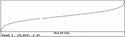
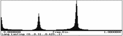
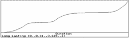
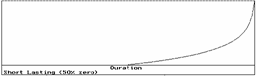
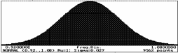
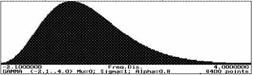
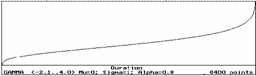
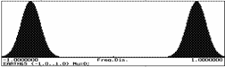
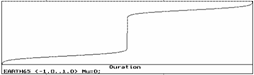
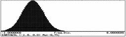
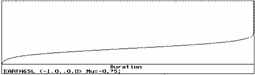
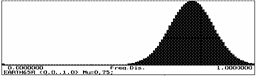
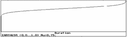
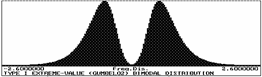
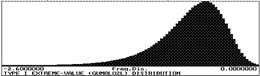
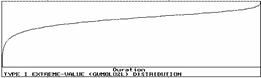
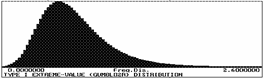
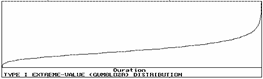
Input random variables are named in Tab. 4. Pertinent nondimensional bounded histograms (excepting histograms Earth65 and Gumbel02) see [5] and [6], where CD is enclosed. Histograms of all input random variables are in Figs. 2-10. Load duration curves, attached to histograms in cases of load distributions, are quantile functions (inverse of distribution functions) and represent the duration of individual load values. Bimodal histogram Earth65 (see also [7]) is composed of histograms Earth65L and Earth65R, as seen in Fig. 8. Bimodal histogram Gumbel02 is composed of histograms Gumbl02L and Gumbl02R, as seen in Fig. 9.

Remark

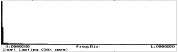
It is appropriate to remind, that individual loads, represented by histograms Dead1, Long2, Short2, Wind1 (and corresponding load duration curves), respect frequency of various magnitudes of loads during the all life of structure. Intervals, when load is zero are also respected, see e.g. histogram Short2, where load is equal zero for the 50% of life of structure.

When Monte Carlo simulation and such histograms are used, the combination of load effects is defined for randomly chosen “arbitrary point in time” of life of structure. Histogram for combinations of load effects is obtained by many times repeated random choice of loads.

The situation is quite different with histograms Earth65 and Gumbel02. These histograms were suggested to simulate extraordinary, extreme loads, such as earthquake, in time of its activity. When histogram Earth65 (or Gumbel02) and mentioned above histograms (Dead1,…Wind1) are used simultaneously, the combination of effects of all loads is analyzed in time interval, which relates to the acting of extraordinary load, e.g. earthquake. Computed probability of failure in such case is evidently much greater then in case, when histogram, used for simulation of extraordinary loading, is refered to the whole life of structure. It results from the fact, that the duration of extraordinary loading (such as earthquake) is extremaly short with respect to the whole life of structure.

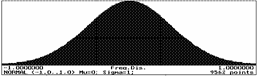
Bounded histogram N1-15 for Young`s modulus E of structural steel is suggested in the rough agreement with mean value 210GPa and standard deviation 12.6GPa, mentioned in [8],[9], or with coefficient of variation of Young`s modulus 0.06 as in [10].

(a)                                                                  (b)

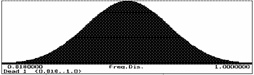
Fig.2 Dead load – (a) Histogram Dead1 and (b) Load Duration Curve

(a)                                                                  (b)

Fig. 3 Long lasting load – (a) Histogram Long2 and (b) Load Duration Curve

(a)                                                                  (b)

Fig. 4 Short lasting load – (a) Histogram Short2 and (b) Load Duration Curve

Table 4 Assigning of dimensionless bounded histograms to input random variables

* File of this histogram is not included in [6]

Moments of discrete random variables (up to fourth moment) are in Table 5.

Table 5 Some properties of probability mass functions

* Large value of the coefficient of variation, mean value is close to zero

** File of the histogram is not included in [6]

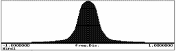
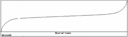
Fig. 5 Wind load – (a) Histogram Wind1 and (b) Load Duration Curve

(a)                                                                  (b)

(c)                                                                  (d)

Fig. 6 Histograms – (a) Normal5  (b) N1-04  (c) N1-08  (d) N1-15

(a)                                                                  (b)

Fig. 7 Temperature difference – (a) Histogram Gamma08 and (b) Load Duration Curve

(a)                                                                  (b)

(c)                                                                  (d)

(e)                                                                  (f)

Fig. 8 Earthquake load – (a) Histogram Earth65 and (b) Load Duration Curve, (c) Histogram Earth65L and (d) Load Duration Curve, (e) Histogram Earth65R and (f) Load Duration Curve.

(a)                                                                  (b)

(c)                                                                  (d)

(e)                                                                  (f)

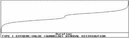
Fig. 9 Earthquake load (a) Histogram Gumbel02 and (b) Load Duration Curve, (c) Histogram Gumbl02L and (d) Load Duration Curve, (e) Histogram Gumbl02R and (f) Load Duration Curve.

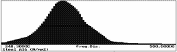
Fig. 10 Yield stress– Histogram A36-m

Probabilistic Reliability Assessment

The simulation-based probabilistic method SBRA and analytical transformation model is applied to the structure in Fig. 1. The performance function (1) (safety function, serviceability function)  Z= R-S  is analyzed using Monte Carlo simulation and M-Starä computer program, see [5], [6].

Safety Assessment (carrying capacity limit state)

Load carrying capacity is evaluated with reference to onset of yielding of the fixed X-X section of column 1. Two types of earthquake loading, represented by histograms Earth65 and Gumbel02 were alternatively applied. Calculated probabilities of failure (probability of exceeding of the yield stress in the outer fiber of the section) are

                        P_f = 0.000028,    when histogram Earth65 is used,

                        P_f = 0.000271,    when histogram Gumbel02 is used,

and

                        P_f  < 1´10^-6,     when earthquake is not considered.

Serviceability Assessment (serviceability limit state)

Serviceability assessment of the structure refers to the lateral displacement limit value d_tol = 40mm of the upper end of the column 1. Two alternative models of earthquake loading are considered again. Computed probabilities of failure (probablity of exceeding of the lateral displacement value 40mm) are

                        P_f = 0.159,    when histogram Earth65 is used

                        P_f = 0.219,    when histogram Gumbel02 is used,

and

                        P_f  = 0.052,     when earthquake is not considered. 

References

[1] VÁCLAVEK, L., Posudek pravdepodobnosti poruchy nevyztuženého rámu s prihlédnutím k montážním imperfekcím, Spolehlivost konstrukcí (sborník referátu konference), Dum techniky Ostrava, spol. s r.o., brezen 2001, in Czech.

[2] VÁCLAVEK, L., MAREK, P., Probabilistic Reliability Assessment of Steel Frame with Leaning Columns, Computational Structural Engineering – An International Journal, Vol.1, No.2, pp. 97-106, 2001.

[3] HALDAR, A., MAHADEVAN, S., Reliability Assessment Using Stochastic Finite Element Analysis, John Wiley & Sons, Inc., 2000.

[4] TEPLÝ, B., NOVÁK, D., Spolehlivost stavebních konstrukcí,Akademické nakladatelství CERM, s.r.o., Brno,1999, in Czech.

[5] MAREK, P., GUŠTAR, M., ANAGNOS, T., Simulation-Based Reliability Assessment for Structural Engineers, CRC Press, Inc., Boca Raton, Florida, 1995.

[6] MAREK, P., BROZETTI, J., GUŠTAR, M., editors, Probabilistic Assessment of Structures using Monte Carlo Simulation. Background, Exercises, Software. Published by ITAM CAS CZ, Prague, Czech Republic, 2001.

[7] MAREK, P., VÁCLAVEK, L.,Issues Related to the Probabilistic Safety Assessment of Steel Structures in the Stability Domain, 15^th ASCE Engineering Mechanics Conference, June 2-5,2002, Columbia University, New York, NY.

[8] TEPLÝ, B., KALA, Z., Reliability Analysis Tools as Applied to the Design of Steel Structures, Engineering Mechanics, Vol. 7, 2000, No.1, pp. 3-13, in Czech.

[9] KALA, Z., KALA, J., Stabiliy  Problems of Steel Beam Structures – a Stochastic Approach, Stavební obzor, Vol.10, 2001, No. 9, pp. 263-266, in Czech.

[10] SOARES GUEDES, C., Uncertainty Modelling in Plate Buckling, Structural Safety, 5, (1988) pp.17-24.